Path Difference (Δx):
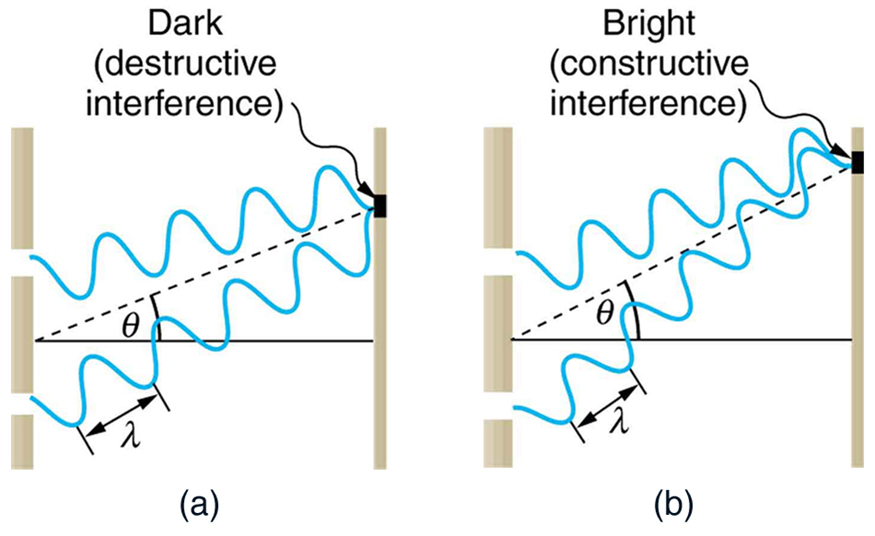
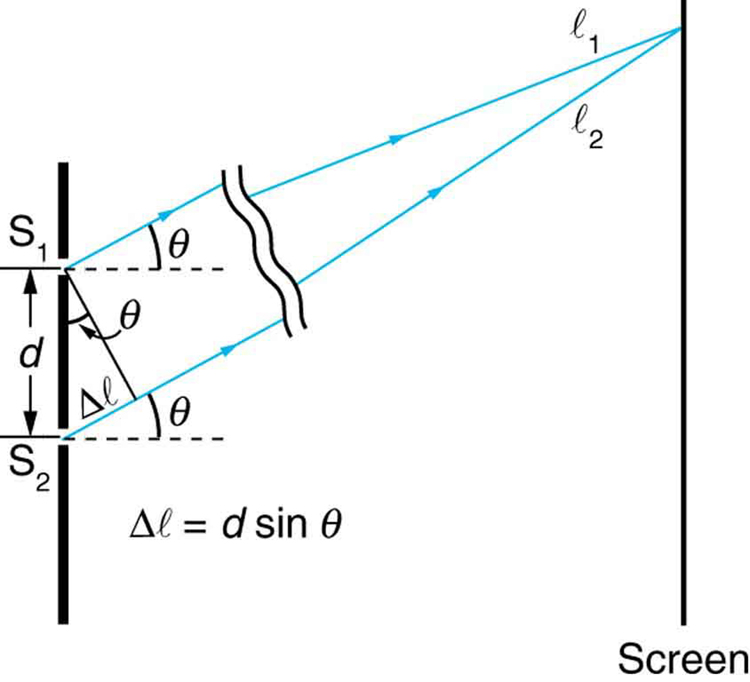
The path difference between two waves reaching a point on the screen from the two slits determines whether they interfere constructively or destructively.
It is given by:
Δx = d sin(θ)
where d is the distance between the slits and θ is the angle between the line joining the point on the screen and the central axis.
Condition for Constructive Interference:
For constructive interference to occur, the path difference Δx must be an integer multiple of the wavelength of the light (λ).
Mathematically, this condition can be expressed as:
Δx = mλ
where m is an integer (0, 1, 2, ...).
Condition for Destructive Interference:
For destructive interference to occur, the path difference Δx must be an odd multiple of half the wavelength of the light (λ/2).
Mathematically, this condition can be expressed as:
Δx = (2m + 1)λ/2
where m is an integer (0, 1, 2, ...).
Intensity Formula:
The intensity \( I \) of light at a point on the screen can be expressed as:
\( I = I_0 \cos^2(\phi) \)
Where:
- \( I_0 \) is the maximum intensity, which occurs when both waves are in phase (constructive interference).
- \( \phi \) is the phase difference between the two waves reaching that point.
The intensity of light at each point depends on the interference pattern, with bright fringes corresponding to constructive interference and dark fringes corresponding to destructive interference.
Phase Difference Formula:
The phase difference \( \phi \) can be related to the path difference \( \Delta x \) using the wave number \( k \) (related to the wavelength \( \lambda \)):
\( \phi = \frac{2\pi}{\lambda} \Delta x \)
So, the intensity at a point on the screen depends on the path difference \( \Delta x \), which in turn depends on the distance from the slits and the angle at which the light reaches that point.
The brightness of the light at different points on the screen in the double-slit experiment is determined by the interference pattern, with bright fringes corresponding to constructive interference and dark fringes corresponding to destructive interference.
The Double-Slit Experiment
In a double-slit experiment, a particle (such as a photon) emitted from a source S can reach a detector D by taking two different paths, e.g., through an upper or a lower slit in a barrier between the source and the detector. After sufficiently many repetitions of this experiment, we can evaluate the frequency of clicks in the detector D and show that it is inconsistent with the predictions based on probability theory. Let us use the quantum approach to show how the discrepancy arises.
The particle emitted from S can reach detector D by taking two different paths, which are assigned probability amplitudes z1 and z2, respectively. We may then say that the upper slit is taken with probability p1 = |z1|² and the lower slit with probability p2 = |z2|². These are two mutually exclusive events. With the two slits open, allowing the particle to take either path, probability theory declares (by the Kolmogorov additivity axiom) that the particle should reach the detector with probability p1 + p2 = |z1|² + |z2|². But this is not what happens experimentally!
That is, if one happens then the other one cannot. For example, "heads" and "tails" are mutually exclusive outcomes of flipping a coin, but "heads" and "6" are not mutually exclusive outcomes of simultaneously flipping a coin and rolling a dice.
Let us see what happens if we instead follow the two "quantum rules": first, we add the amplitudes, then we square the absolute value of the sum to get the probability. Thus, the particle will reach the detector with probability
\( p = |z|^2 \)
\( = |z_1 + z_2|^2 \)
\( = |z_1|^2 + |z_2|^2 + z_1^* z_2 + z_1 z_2^* \)
\( = p_1 + p_2 + |z_1| \cdot |z_2| (e^{i(\phi_2 - \phi_1)} + e^{-i(\phi_2 - \phi_1)}) \)
\( = p_1 + p_2 + 2p_1 p_2 \cos(\phi_2 - \phi_1) \)
The appearance of the interference terms marks the departure from the classical theory of probability. The probability of any two seemingly mutually exclusive events is the sum of the probabilities of the individual events modified by the interference term. Depending on the relative phase φ2 - φ1, the interference term can be either negative (destructive interference) or positive (constructive interference), leading to either suppression or enhancement, respectively, of the total probability p.
The algebra is simple; our focus is on the physical interpretation. Firstly, note that the important quantity here is the relative phase φ2 - φ1 rather than the individual phases φ1 and φ2. This observation implies that the particle reacts only to the difference of the two phases, each pertaining to a separate path. Secondly, what has happened to the additivity axiom in probability theory? What was wrong with it? One problem is the assumption that the processes of taking the upper or the lower slit are mutually exclusive; in reality, as we have just mentioned, the two transitions both occur simultaneously.
According to the philosopher Karl Popper (1902–1994), a theory is genuinely scientific only if it is possible, in principle, to establish that it is false. Genuinely scientific theories are never finally confirmed because, no matter how many confirming observations have been made, observations that are inconsistent with the empirical predictions of the theory are always possible. There is no fundamental reason why Nature should conform to the additivity axiom.
We find out how nature works by making "intelligent" guesses, running experiments, checking what happens, and formulating physical theories. If our guess disagrees with experiments, then it is wrong, so we try another intelligent guess, and another, etc. Right now, quantum theory is the best guess we have: it offers good explanations and predictions that have not been falsified by any of the existing experiments. This said, rest assured that one day quantum theory will be falsified, and then we will have to start guessing all over again.
Three Polarizing Filters — interactive (Malus's law)
A laser sends light through three polarizers in a row. With filter A vertical (0°) and filter C horizontal (90°), no light gets through. Insert filter B at 45° between them and light reappears — because a polarizer doesn't just block, it re-projects the polarization. Each stage follows Malus's law I = I₀ cos²(Δθ).
Meter reading: 12.5% of the source (25.0% of the light that passed filter A)
Third-Polarizing-Filter Experiment Demystified — How It Works
Shine light through two polarizing filters oriented at 90° to each other, and no light gets through. But put a third filter inbetween them, at 45° to each of the existing filters, and amazingly enough — some lights gets through!
This popular experiment is often described as “strange.” It is usually presented in the context of quantum mechanics, as an example of the “spookiness” of quantum effects. Rarely, however, does the presenter inform the audience that this experiment can be explained in very simple terms of cause and effect, without reference to spooky quantum magic or anything like that.
Let’s start by going over the standard experiment:
Figure 1
In Figure 1, an unpolarized, parallel light source is fired through a polarizing filter, and the light strongly registers in a light meter at the other end.
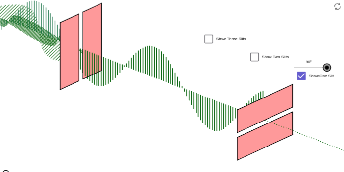
Figure 2
In Figure 2, a second filter is introduced, oriented at 90° to the first one. Now, no light gets through.
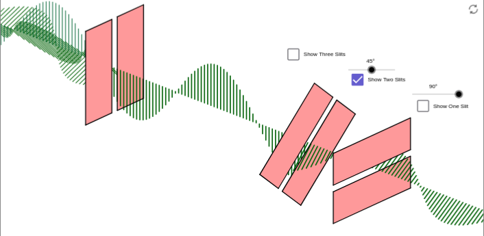
Figure 3
In Figure 3, a third filter is placed inbetween the first two, at 45° to each of them. Suddenly, the light meter registers a significant amount of light, although not as much as in Figure 1. Spooky!
Spookiness and the Word “Filter”
Why do these results seem spooky? The reason is because of the misapplication of the word “filter.” A filter is commonly understood to mean a device that knocks some items out of a stream, while leaving others essentially untouched. A good example of a filter is a sieve — it blocks objects of a particular size, while allowing objects of other sizes to pass through.
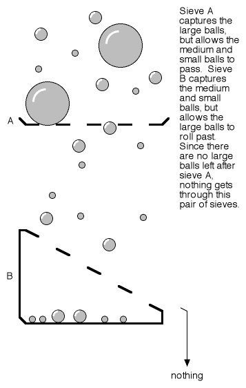
Figure 4
Another example would be a color filter that knocks out some frequencies of light while letting others through.
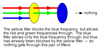
Figure 5
Understood this way, the results of the polarizer experiment are indeed spooky. If the all-blocking equivalent of Figure 2 is constructed using sieves or color frequency filters (see Figures 4 and 5), we are certainly confident that the addition of more filters in the middle of the sequence will not yield different results at the end.
But what if our so-called “filters” could not only block components of the stream, but also change them? Then we would not be surprised at all if the addition of new “filters” in the middle caused items to get through to the end. If a sieve could not only block particles, but also change their size, or if a color filter could not only block frequencies, but shift light to a different frequency, then all bets are off.
This, in fact, is what a polarizer does.
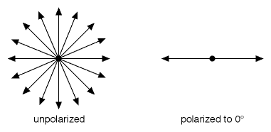
Figure 6
Look at Figure 6 and ask yourself this question: What percentage of the unpolarized light is oriented to exactly 0° or very nearly 0°? Almost none of it — certainly less than 1%. So, if a polarizer simply knocked out undesirable orientations, the strength of the remaining light would be almost entirely gone — it would be less than 1% as strong as the original light source. But you know a polarizer doesn’t do that, because you can pick up an ordinary pair of polarizing sunglasses and observe that they’re not even particularly dark! Obviously, something else must be happening.

Figure 7
Let’s see what happens to each of the orientations represented in our simple diagram (from Figure 6):

Figure 8
In Figure 8, we see that light already at 0° is unchanged. We knew that already.
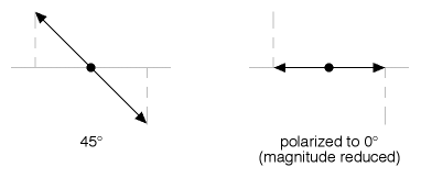
Figure 9
In Figure 9, we see what happens to light oriented at 45° — it has its transverse (vertical) component destroyed, and becomes oriented to 0°, but with a weaker magnitude. Simple geometry tells us that it must have a magnitude about 71% of what it had before being polarized to 0° — i.e., 1/sqrt(2) = .707
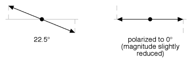
Figure 10
Figure 10 shows us that light that is close to 0° loses only a little of its magnitude when being crushed to 0°...
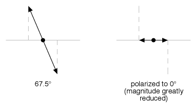
Figure 11
...while Figure 11 shows us that light that is close to 90° off of the polarizer loses most of its magnitude when being crushed to 0°.
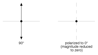
Figure 12
And finally, Figure 12 illustrates light at 90° to the filter being crushed completely out of existence. Figure 12, in fact, illustrates what is happening in Figure 2 when we had only two polarizers in the path of our light source.
What is happening in Figure 3? With our new understanding of what a polarizer does, it is easy to figure it out:
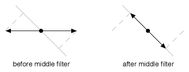
Figure 13
Figure 13 shows the middle filter taking 0° polarized light (from the first filter) and crushing it to a 45° orientation. This causes the light to drop to about 71% of its magnitude coming from the first filter.
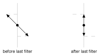
Figure 14
And Figure 14 shows the last filter taking the 45° polarized light (from the middle filter) and crushing it to a 90° orientation. This causes another 29% drop (0.71x) in magnitude, for an overall drop of exactly 50% (as compared to the results of the single-filter setup in Figure 1). These results can be verified by performing the experiment with an actual light meter — the meter should show about twice as strong a reading in the Figure 1 arrangement as it does in the Figure 3 arrangement.
So there you have it! No spooky quantum properties. Nothing very mysterious about it, in fact. A straightforward chain of cause and effect, yielding rational, comprehensible results.
Sequential Stern–Gerlach
A beam of spin-½ atoms is first prepared spin-up along Z by the left magnet. A second Stern–Gerlach magnet is rotated by an angle θ relative to the first. Classically you would expect a continuous smear; quantum mechanics predicts the beam splits into exactly two discrete spots, with probabilities cos²(θ/2) (up) and sin²(θ/2) (down).
▲ P(up) = 0.85 ▼ P(down) = 0.15
The Stern–Gerlach Experiment
In 1922, Otto Stern and Walther Gerlach sent a beam of silver atoms through a strong, inhomogeneous magnetic field. Each atom carries a magnetic moment, so classically the field should deflect atoms by an amount proportional to the component of that moment along the field — and since the moments point in every direction, the beam should spread into a single continuous smear on the detector.
Instead, the beam split into two discrete spots. The component of angular momentum along the measurement axis is quantised: for a spin-½ particle it can only take the values \( +\tfrac{\hbar}{2} \) (“up”) or \( -\tfrac{\hbar}{2} \) (“down”).
Sequential measurements — what the simulator shows
Prepare an atom to be spin-up along Z using a first apparatus. Now measure it again with a second Stern–Gerlach magnet whose axis \( \hat{n} \) is rotated by an angle \( \theta \) from Z. The state \( |{\uparrow_z}\rangle \) written in the basis of the tilted apparatus is:
\( |{\uparrow_z}\rangle = \cos\tfrac{\theta}{2}\,|{\uparrow_n}\rangle + \sin\tfrac{\theta}{2}\,|{\downarrow_n}\rangle \)
so the probabilities of the two outcomes are given by the Born rule:
\( P(\uparrow_n) = \cos^2\!\tfrac{\theta}{2}, \qquad P(\downarrow_n) = \sin^2\!\tfrac{\theta}{2} \)
- θ = 0°: the two magnets agree — every atom comes out “up” (P = 1). The result is repeatable.
- θ = 90°: a Z-up atom has no definite value along the new axis; the outcome is a perfect 50/50 coin flip. Measuring along X has also erased the original Z information.
- θ = 180°: the second magnet is upside-down, so “up” and “down” swap — every atom now comes out “down” (P = 1).
The half-angle \( \theta/2 \) is the fingerprint of spin-½: you must rotate the apparatus by a full \( 360^\circ \) — not \( 180^\circ \) — to return to the original probabilities. This experiment is the cleanest demonstration that measurement in quantum mechanics is probabilistic, that observables can be incompatible, and that a measurement changes the state it acts on.
Ramsey Interferometer — separated oscillatory fields
A two-level atom starts in the ground state. Two π/2 pulses, separated by a free-evolution time T, drive it. During T the atomic phase advances at the detuning δ (= drive frequency − atomic frequency). The chance of finding the atom excited oscillates as Pe(δ) = cos²(δT/2) — the Ramsey fringes below. Longer T makes the fringes finer, which is exactly why Ramsey's method underpins atomic clocks.
At δ = 0: P(excited) = 1.000
The Ramsey Interferometer
Norman Ramsey's method of separated oscillatory fields (1949, Nobel Prize 1989) is the technique at the heart of every atomic clock. Instead of driving a two-level atom with one long pulse, it uses two short \( \pi/2 \) pulses separated by a period of free evolution of duration \( T \). It is a quantum interferometer in which the two “paths” are the ground and excited states of the atom.
How it works
- The atom begins in the ground state \( |g\rangle \).
- The first \( \pi/2 \) pulse places it in an equal superposition \( \tfrac{1}{\sqrt{2}}(|g\rangle + |e\rangle) \) — on the Bloch sphere the state now lies on the equator.
- During the free time \( T \), the superposition precesses. If the drive is detuned from the atomic frequency by \( \delta \), the two components accumulate a relative phase \( \phi = \delta T \).
- The second \( \pi/2 \) pulse converts that accumulated phase into a population difference that a detector can read out.
The probability of finding the atom in the excited state is:
\( P_e(\delta) = \cos^2\!\left(\dfrac{\delta T}{2}\right) = \tfrac{1}{2}\big(1 + \cos(\delta T)\big) \)
Plotting \( P_e \) against the detuning \( \delta \) gives the Ramsey fringes shown in the simulator. Their spacing is \( \Delta\delta = 2\pi / T \): the longer the free-evolution time T, the narrower the central fringe, and the more precisely the drive frequency can be locked to the atomic transition. This is why a longer interrogation time means a more accurate clock.
Compared with driving a single long pulse (a Rabi measurement), Ramsey's separated-pulse scheme is far less sensitive to fluctuations in the pulse amplitude and to the field's uniformity, because the atom spends most of its time evolving freely rather than being driven — which is what makes it so precise.